jpy_usd <-
  "JPY=X" %>%
  tq_get(from = "2000-01-01")

jpy_usd %>%
  ggplot(aes(x = date, y = high)) +
  geom_line(color = "steelblue") +
  theme_minimal() +
  scale_y_continuous(
    labels = dollar_format(
      suffix = "",
      prefix = "\u00a5"
    )
  ) +
  scale_x_date(
    date_breaks = "3 years",
    date_labels = "%Y"
  ) +
  labs(
    x = "",
    y = "",
    title = "JPY to USD"
  ) +
theme(plot.title = element_text(hjust = .5))Exchange Rates
Introduction
In our Chapter on interest rates, we noted that interest rates can be thought of as the most important price in the world, the price of money or the price of time. The interest rate policy set by the Fed impacts the price of money for the U.S. Dollar but also for other currencies in the world because any currency can be priced in terms of another currency, this is what an exchange rate represents. When the Fed alters the price of the U.S. Dollar through its interest rate choices, the relative price of other currencies is also affected. Given that the U.S. Dollar is the reserve currency for the world (i.e. the currency against which other currencies are measured), any action by the Fed carries important implications for exchange rates.1
For an example, let’s have a look at the exchange rate between the Japanese Yen (JPY) and the U.S. Dollar (USD). When we talk about exchange rates, it’s important to note that there are two ways to express them: how many JPY does it take to buy 1 USD; or, how many USD does it take to buy 1 JPY. The convention in exchange rates is to express currency quotes as BASE/QUOTE where you receive 1 unit of the BASE currency for a variable amount of the QUOTE currency. For example, if we have USD/JPY = 135 it means you can exchange 1 USD for 135 JPY; of course we would also have JPY/USD = 1/135.2 Most exchange rate quotes use the USD as the base currency though notable exceptions are the Euro (EUR) and the British Pound (GBP).
Small technical note: to get the Yen symbol on our Y-axis, we need to find the unicode character code for yen, which is “u00a5”.
Let’s have a look at recent Yen movement. We use the ’tq_get()` function to pull this data from yahoo! Finance.
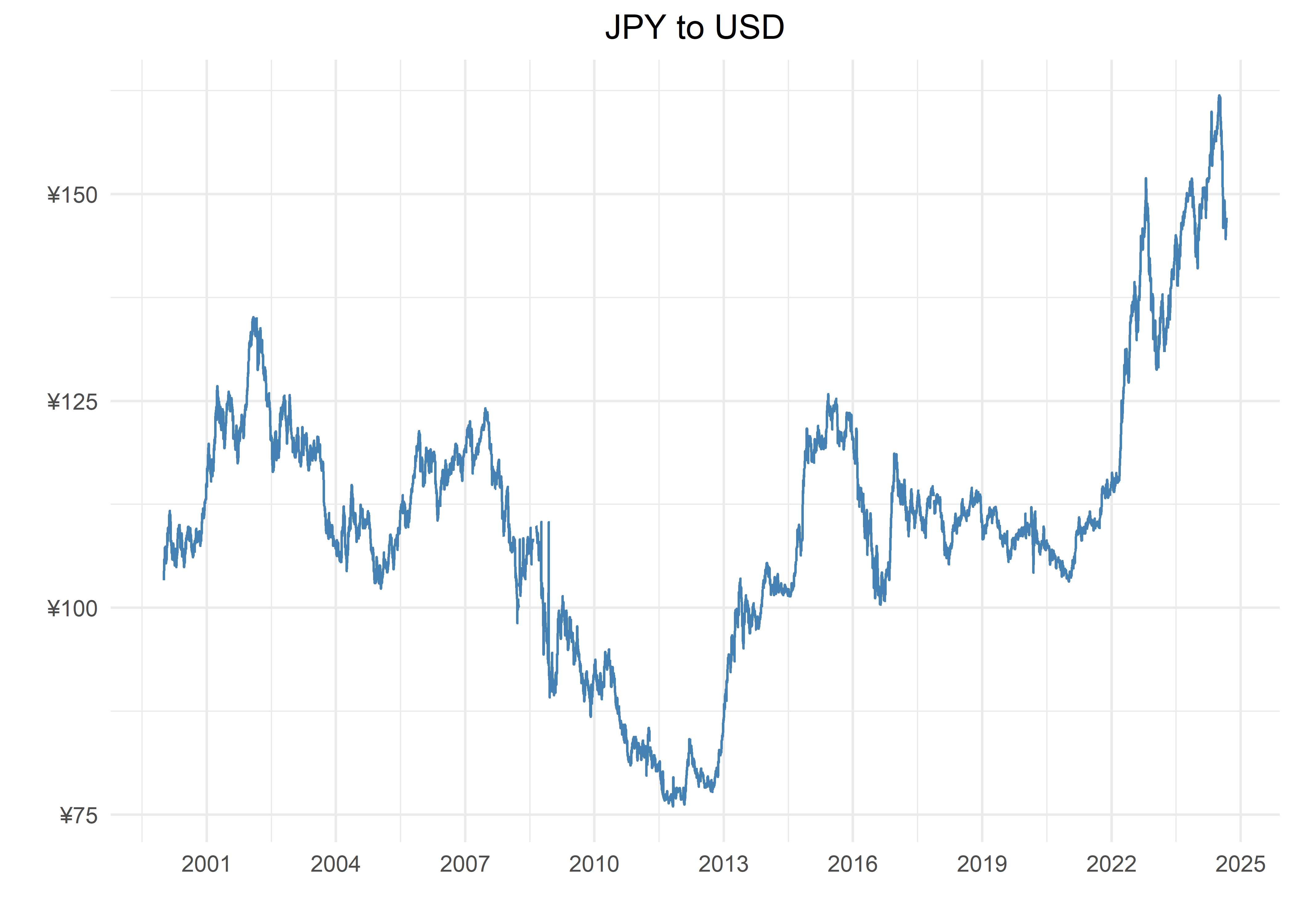
The Yen reached a twenty-year low, or the dollar reached a twenty-year high in Yen terms 2024. The US Fed was raising interest rates as this time (as we have discussed) and the Japanese Central Bank - the Bank of Japan or the BOJ - kept low interest rates. Those diverging rates makes USD more attractive relative to Yen.
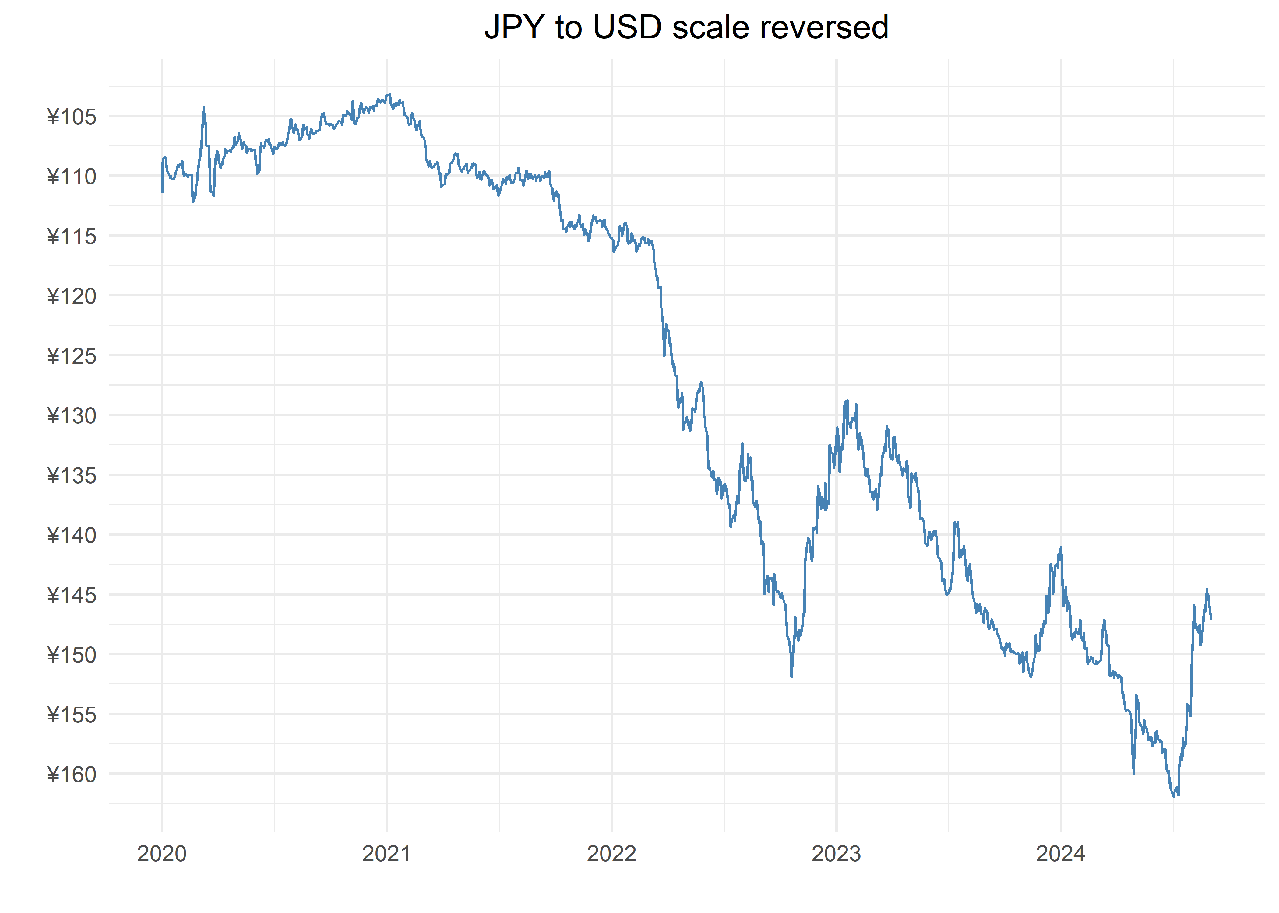
Note that exchange rate charts are somewhat peculiar. The USD/JPY rate almost halves from 2002 until 2012. If this was a stock price chart we would conclude the JPY struggled mightily during this period, but because this an exchange rate where the JPY is the quote currency it actually means the JPY outperformed the USD. Back in 2002, 1 USD bought about 135 JPY, but by 2012 1 USD could only buy about 75 JPY; we say the JPY strengthened against the USD. For this reason, exchange rate plots sometimes have an inverted scale in the y-axis, so that when the quote currency strengthens the plot goes up instead of down. We can easily code an inverted scale in ggplot by using the scale_y_reverse() function, as we do below.
jpy_usd %>%
  filter(date >= "2020-01-01") %>%
  ggplot(aes(x = date, y = high)) +
  geom_line(color = "steelblue") +
  theme_minimal() +
  labs(
    x = "",
    y = "",
    title = "JPY to USD scale reversed"
  ) +
  scale_y_reverse(
    labels = dollar_format(
      suffix = "",
      prefix = "\u00a5"
    ),
    breaks = pretty_breaks(10)
  ) +
  scale_x_date(
    date_breaks = "1 years",
    date_labels = "%Y"
  ) +
  theme(plot.title = element_text(hjust = .5))
We could build this chart for any currency pair and think about what the price is communicating about relative interest rates but let’s move on to exploring the value of the USD in general, not against a specific currency. For that we turn to a widely followed dollar index called the DXY, which tracks the value of the USD against a weighted basket of other currencies. When we hear pundits talk about the ‘strength of the dollar’, it is usually in reference to this index.
Here are the packages we will be using in this chapter:
# workhorse packages
library(tidyverse)
library(tidyquant)
library(timetk)
library(readxl)
library(janitor)

# data sources
library(fredr)
library(riingo)

# vis specific
library(gt)
library(plotly)
library(scales)
The DXY
The most widely cited index of the US Dollar priced in other currencies is called the DXY (sometimes pronounced the ‘dixy’). The DXY is the creation of a private company, the Inter-Continental Exchange (the ICE) and is the most widely cited dollar index.3
Conclusion
Footnotes
Readers with an Economics academic background will recall that one of the foundational theories of exchange rate determination is the interest rate parity.↩︎
More information on the basics of the foreign exchange market can be found in the CME’s Introduction to FX lessons at https://www.cmegroup.com/education/courses/introduction-to-fx/what-is-fx.html↩︎
For more background on how the DXY is constructed, please see this methodology piece from the ICE https://www.theice.com/publicdocs/data/ICE_FX_Indexes_Methodology.pdf.↩︎

