# workhorse packages
library(tidyverse)
library(tidyquant)
library(timetk)
library(readxl)
library(janitor)

# data sources
library(fredr)

# vis specific
library(gt)
library(gtExtras)
library(ggrepel)
library(ggtext)
library(plotly)
library(scales)
library(formattable)The Federal Reserve
Introduction
The Federal Reserve (Fed) was established by Congress back in 1913. The Federal Reserve Act provided “for the the establishment of Federal Reserve Banks, to furnish an elastic currency, to afford means of rediscounting commercial paper, to establish a more effective supervision of banking in the United States, and for other purposes.”1 The Fed has a dual mandate to enact policies that promote price stability and maximum sustainable employment. Though not an explicit mandate, since the global financial crisis (GFC) of 2008-2009 the Fed has been concerned with financial stability and this has led to the creation of many novel programs, such as the Troubled Assets Relief Program (TARP) and the Large-Scale Asset Purchases (commonly called quantitative easing).
The size of the Fed in the economy has increased dramatically since the GFC. In this chapter we take a closer look at the balance sheet of the Fed, its assets and liabilities, and the impact of changes to the Fed’s preferred interest rate. In the first part of this chapter, we will focus on just the Assets side of the Fed’s balance sheet, how it adds or subtracts liquidity from the financial system and how it ultimately leads to easing or tightening financial conditions. Then, we will look at the Liabilities side of the balance sheet and the Fed is using a novel instrument, reverse repurchase agreements, to fine tune its policy. Finally, we will take another look at the Federal Reserve’s main tool for fine-tuning monetary policy, the Federal Funds rate.
How does monetary policy affect the economy? Traditional macroeconomic models posit that monetary policy works primarily through three neo-classical channels:
- cost-of-capital effects,
- wealth effects, and
- exchange-rate
Consider a situation where the central bank raises interest rates in order to prevent the economy from overheating. Consequently, the following may happen
- First, increase in the cost of capital nay dissuade capital investments by firms and purchases of houses and durables by consumers.
- Second, higher rates will reduce the present value of various assets and the resulting wealth effects will lower aggregate spending.
- Third, higher rates may strengthen the domestic currency, depressing net exports.
In addition, a more modern view recognizes the importance of frictions in financial markets, so that monetary policy may also affect economic activity via so-called credit channel. There may be frictions in raising capital. For example, a tighter policy reduces both the net worth and the cash flow of firms, and these balance-sheet effects make it more expensive for them to obtain external financing, thereby depressing firm investment.
Readers interested in the intricacies of central banking would do well to read The Fed Guy Blog by former Fed trader Joseph Wang or his book Central Banking 101 where he explains how the Fed transforms words into actions. This chapter is an attempt to visualize and make concrete changes in the the Fed balance sheet, so we can track the end result of Fed actions.
With that, let’s get into the Federal Reserve.
Here are the packages we will be using in this chapter:
Fed Balance Sheet: the Assets Side
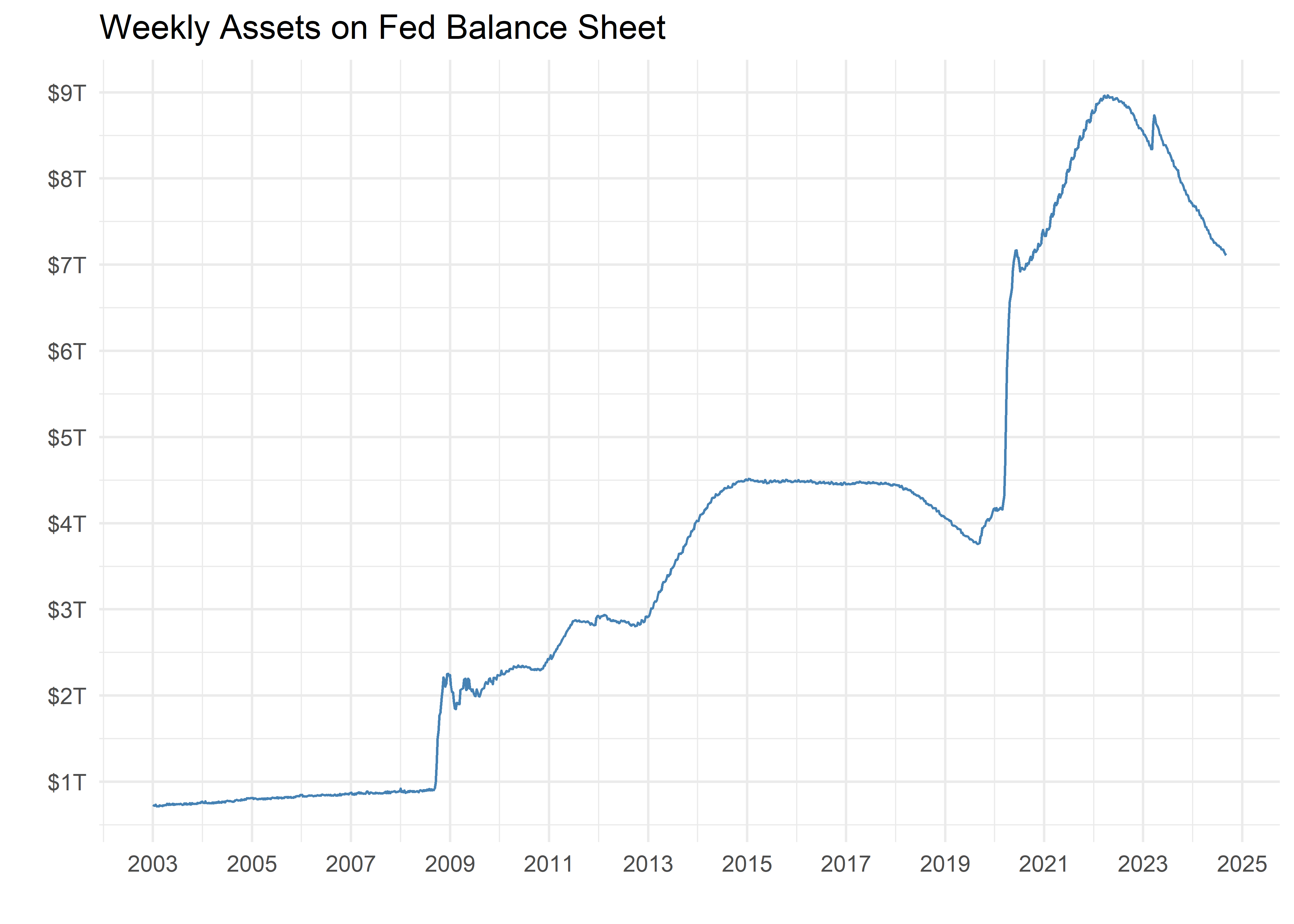
In addition to interest rate targeting via the Federal Funds Rate, the Fed can affect overall financial liquidity through it’s balance sheet. The Fed can expand its balance sheet almost without limit because it buys securities from primary dealers and pays them with excess reserves, which is just a number in the Fed’s ledger. Fortunately, the Fed publishes a weekly update about its balance sheet every Thursday, in Factors Affecting Reserve Balances Table H.4.1 and FRED also publishes the time series of that data. For starters, let’s pull the weekly level of total assets (in millions of dollars) in the Fed’s balance sheet.
fed_assets_on_bs <-
  "WALCL" %>%
  tq_get(
    get = "economic.data",
    from = "2003-01-01"
  )

fed_assets_on_bs %>%
  ggplot(aes(x = date, y = price)) +
  geom_line(color = "steelblue") +
  labs(
    title = "Weekly Assets on Fed Balance Sheet",
    x = "",
    y = ""
  ) +
  scale_y_continuous(
    labels = dollar_format(
      scale = 1 / 1000000,
      suffix = "T"
    ),
    breaks = pretty_breaks(10),
  ) +
  scale_x_date(
    date_breaks = "2 years",
    date_labels = "%Y"
  ) +
  theme_minimal()
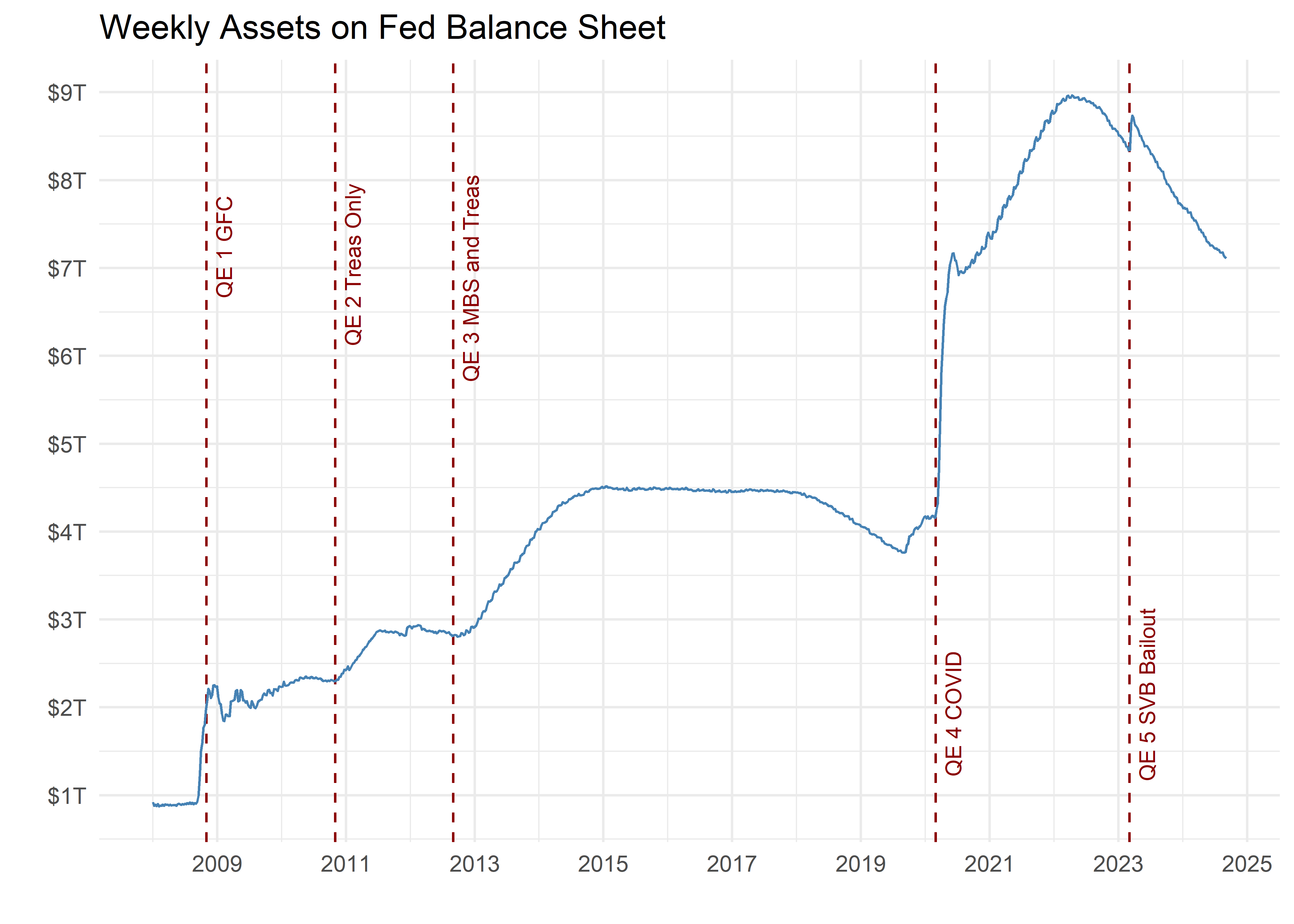
The next chart shows the same trend in assets, but we have also labeled 5 stages of Quantitative Easing since 2008. Quantitative Easing (QE) occurs when the Fed eases financial conditions not by lower the Fed Funds Rate but by purchasing assets.
The five labeled QE stages are:
- GFC - the financial crisis from whence QE originated
- Treasuries only - when the Fed bought only Treasuries
- MBS and Treasury - when the Fed expanded to buying mortgage-backed securities
- COVID - when the Fed undertook emergency QE during the pandemic economic shutdown
- SVB Bailout
fed_assets_on_bs %>%
  filter(date >= "2008-01-01") %>%
  ggplot(aes(x = date, y = price)) +
  # geom_line(color = "steelblue") +
  labs(
    title = "Weekly Assets on Fed Balance Sheet",
    x = "",
    y = ""
  ) +
  geom_textvline(
    xintercept =
      as.integer(ymd("2008-11-01")),
    label = "QE 1 GFC",
    hjust = 0.8,
    linetype = 2,
    size = 3,
    vjust = 1.3,
    color = "darkred"
  ) +
  geom_textvline(
    xintercept =
      as.integer(ymd("2010-11-01")),
    label = "QE 2 Treas Only",
    hjust = 0.8,
    linetype = 2,
    size = 3,
    vjust = 1.3,
    color = "darkred"
  ) +
  geom_textvline(
    xintercept =
      as.integer(ymd("2012-09-01")),
    label = "QE 3 MBS and Treas",
    hjust = 0.8,
    linetype = 2,
    size = 3,
    vjust = 1.3,
    color = "darkred"
  ) +
  geom_textvline(
    xintercept =
      as.integer(ymd("2020-03-01")),
    label = "QE 4 COVID",
    hjust = 0.1,
    linetype = 2,
    size = 3,
    vjust = 1.3,
    color = "darkred"
  ) +
  geom_textvline(
    xintercept =
      as.integer(ymd("2023-03-05")),
    label = "QE 5 SVB Bailout",
    hjust = 0.1,
    linetype = 2,
    size = 3,
    vjust = 1.3,
    color = "darkred"
  ) +
  geom_line(color = "steelblue") +
  scale_y_continuous(
    labels = dollar_format(
      scale = 1 / 1000000,
      suffix = "T"
    ),
    breaks = pretty_breaks(10),
  ) +
  scale_x_date(
    date_labels = "%Y",
    date_breaks = "2 years"
  ) +
  theme_minimal()
Fed Balance Sheet: the Liabilities Side
Fed Liquidity and Markets
FOMC Announcements and Market Returns
Impact on Market Returns
Conclusion
Footnotes
A brief history of the creation of the Fed can be found at https://www.newyorkfed.org/aboutthefed/history_article.html.↩︎

