Interest Rates

Introduction

In the following chapter, we discuss interest rates and their relationship to economic and market conditions. We also introduce a few key skills in the area of economic data science: creating, exploring and analyzing different time series based features like lags and rolling calculations. Lag and rolling effects of macroeconomic features go beyond interest rates and we hope the workflows we establish in this chapter have broad applicability, in economics and in general financial analytics.

The structure of our interest rate chapter is as follows: we start with a brief summary of interest rates and Treasury debt instruments (or Treasuries) and why they matter for markets and the economy. We then import and visualize data on Treasuries. Next we create different time-based features based on our imported Treasury data, and we close with a few interest rates use cases. Let’s get it!

Interest rates are the price that borrowers (or debtors) must pay to lenders (or creditors) for access to capital today in exchange for a promise to repay that capital in the future. Interest rates are a function of supply and demand from creditors and debtors, overall economic conditions, inflation and central bank actions. Interest rates have been called both the price of money and the price of time, and also the most important price in the world.¹

In fact, Ray Dalio, the founder of Bridgewater Capital, hypothesizes the following crucial and causal connection between interest rates (the cost of credit) and recessions:

“Recessions occur when central banks raise the cost of credit…recessions end when central banks lower interest rates.”²

Another of our favorite market thinkers Howard Marks ascribes much of the stupendous performance of the stock market between 1980 and 2021 to the fact that this period was marked by low and declining interest rates. In one of his investment letters titled “Sea Change”, he listed some of the effects of low interest rates way.³

Accelerate the growth of the economy by making it cheaper for consumers to buy on credit and for companies to invest
Provide a subsidy to borrowers (at the expense of lenders and savers)
Increase the fair value of assets…as interest rates fall, valuation parameters such as p/e ratios and enterprise values rise, and cap rates on real estate decline
Create a “wealth effect” that makes people feel richer and thus more willing to spend
Produce a bonanza for those who buy assets using leverage

Mr. Marks further foresees a “Sea Change” that started in 2022 and will characterize a different interest rate and inflation environment. He opines, “Inflation and interest rates are highly likely to remain the dominant considerations influencing the investment environment for the next several years.”⁴

Well, we could continue quoting others on the importance of interest rates, but suffice it to say they are very important to the economy and financial markets.

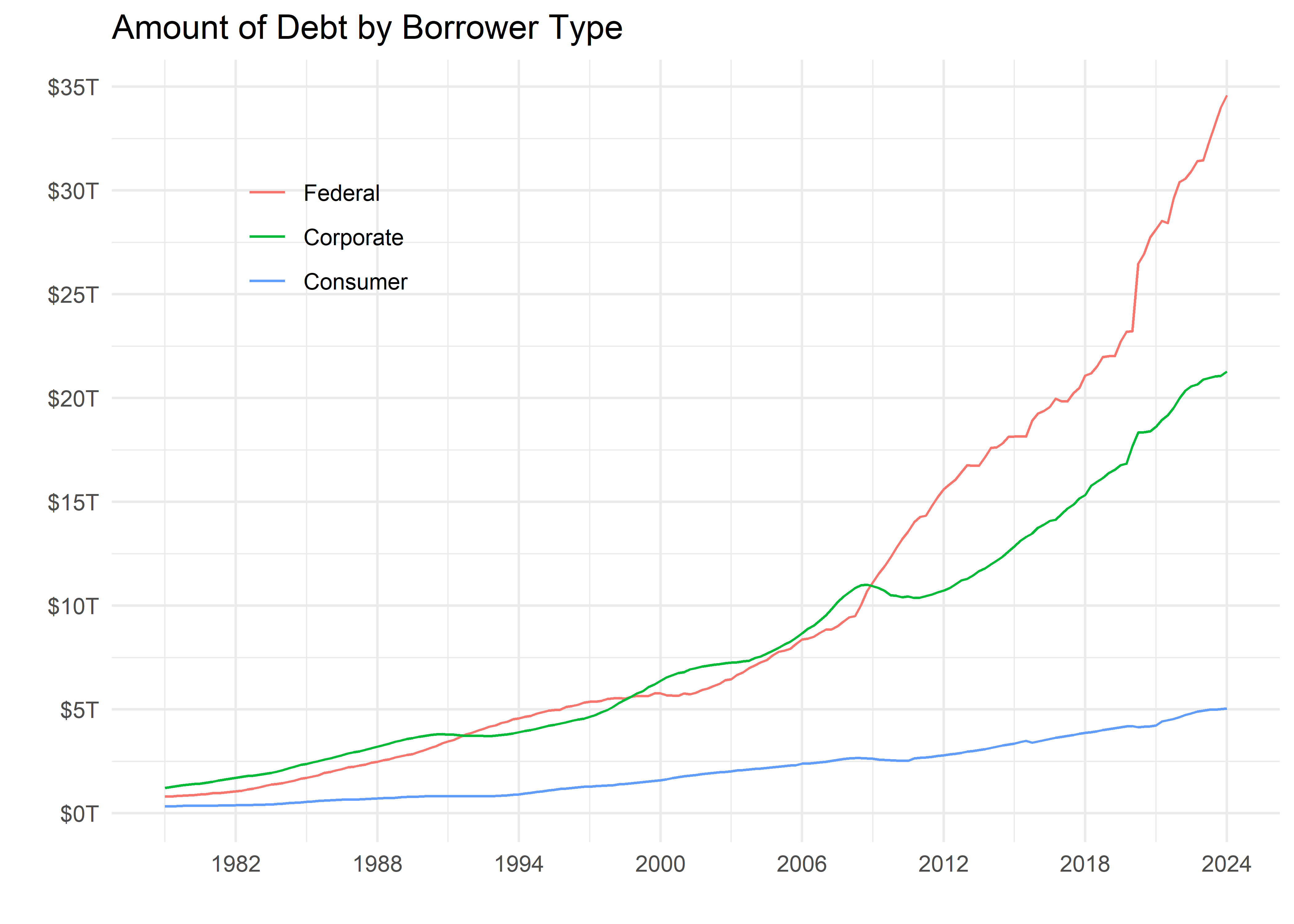
Since interest is the cost of debt, before we even look interest rates, let’s have a quick exploration of three types of debt, each of which has dramatically increased since the early 1980’s and each of which incurs a cost or interest rate.

debt_tibble <- tibble(
  symbol = c("GFDEBTN", "TBSDODNS", "HCCSDODNS"),
  name = c("Federal", "Corporate", "Consumer") %>% as_factor()
)

debt_tibble %>%
  tq_get(get = "economic.data", from = "1979-01-01") %>%
  mutate(
    price =
      case_when(
        symbol == "GFDEBTN" ~ price / 1000000,
        T ~ price / 1000
      )
  ) %>%
  ggplot(aes(
    x = date, y = price,
    color = name
  )) +
  geom_line() +
  scale_y_continuous(
    labels = dollar_format(
      suffix = "T"
    ),
    breaks = pretty_breaks(10)
  ) +
  scale_x_date(
    date_breaks = "6 years",
    date_labels = "%Y"
  ) +
  theme_minimal() +
  labs(
    x = "", y = "",
    title = "Amount of Debt by Borrower Type",
    color = ""
  ) +
  theme(
    legend.position = c(.2, .8),
    legend.margin = margin(0, 0, 0, -15),
    legend.box.margin = margin(-5, -5, -5, -5)
  )

When we glance at that chart, we see that since 1980 corporate debt has increased more than 10x, Federal debt has increased more than 30x and consumer debt has increased about 5x. Interest rates are the price of all that debt.

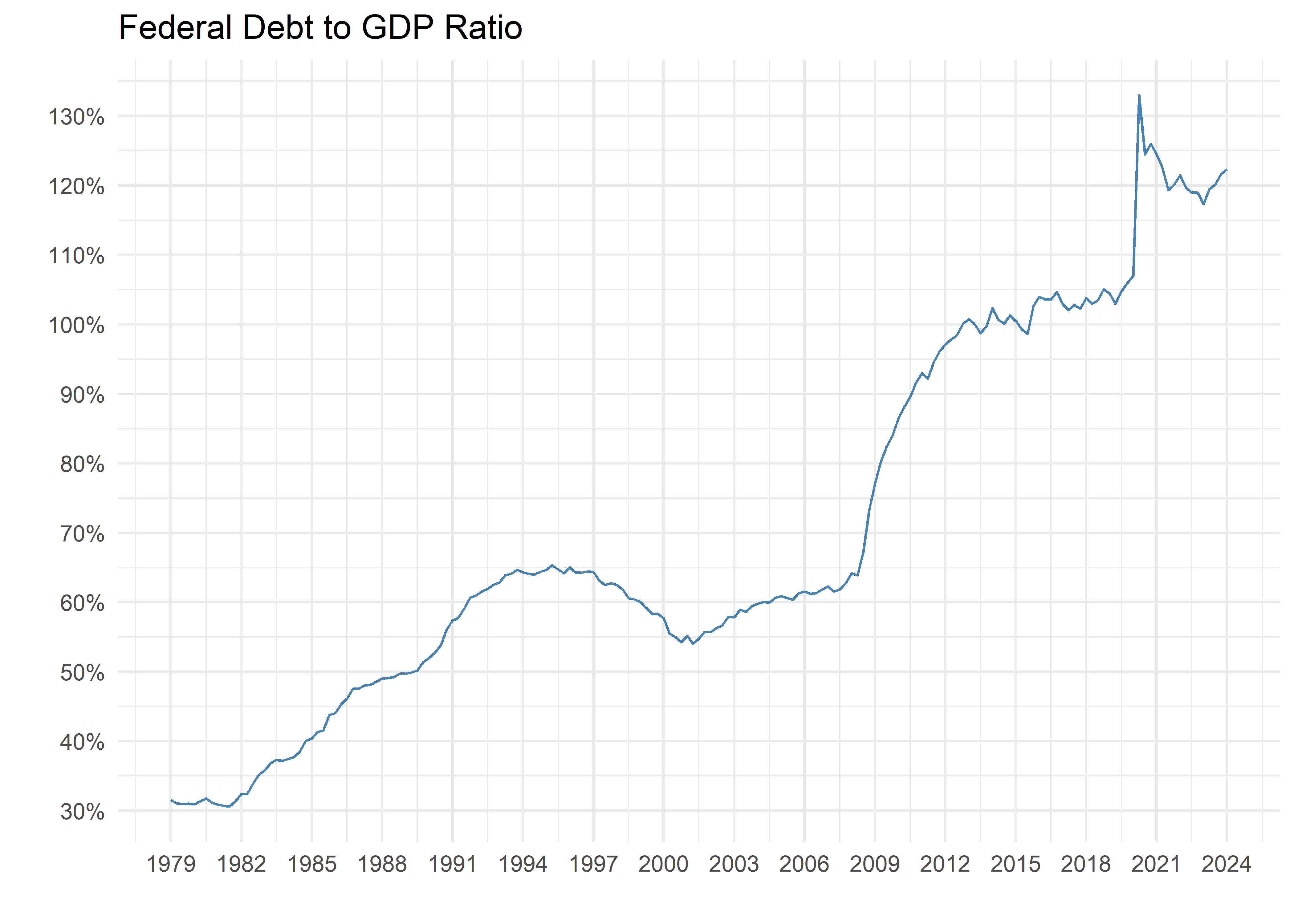
It is important to contextualize those charts in terms of GDP, because the economy has also grown over this time. Here is the Federal Debt-to-GDP Ratio.

"GFDEGDQ188S" %>%
  tq_get(get = "economic.data", from = "1979-01-01") %>%
  ggplot(aes(x = date, y = price)) +
  geom_line(color = "steelblue") +
  scale_y_continuous(
    labels = percent_format(
      scale = 1
    ),
    breaks = pretty_breaks(10)
  ) +
  scale_x_date(
    date_breaks = "3 years",
    date_labels = "%Y"
  ) +
  theme_minimal() +
  labs(
    x = "", y = "",
    title = "Federal Debt to GDP Ratio"
  )

Not quite a 30x increase in the ratio, but we have gone from Federal Debt being around 30% of GDP to around 120% of GDP. The inflection points seem to be recent crises: the GFC and COVID era both saw large spikes in this ratio.

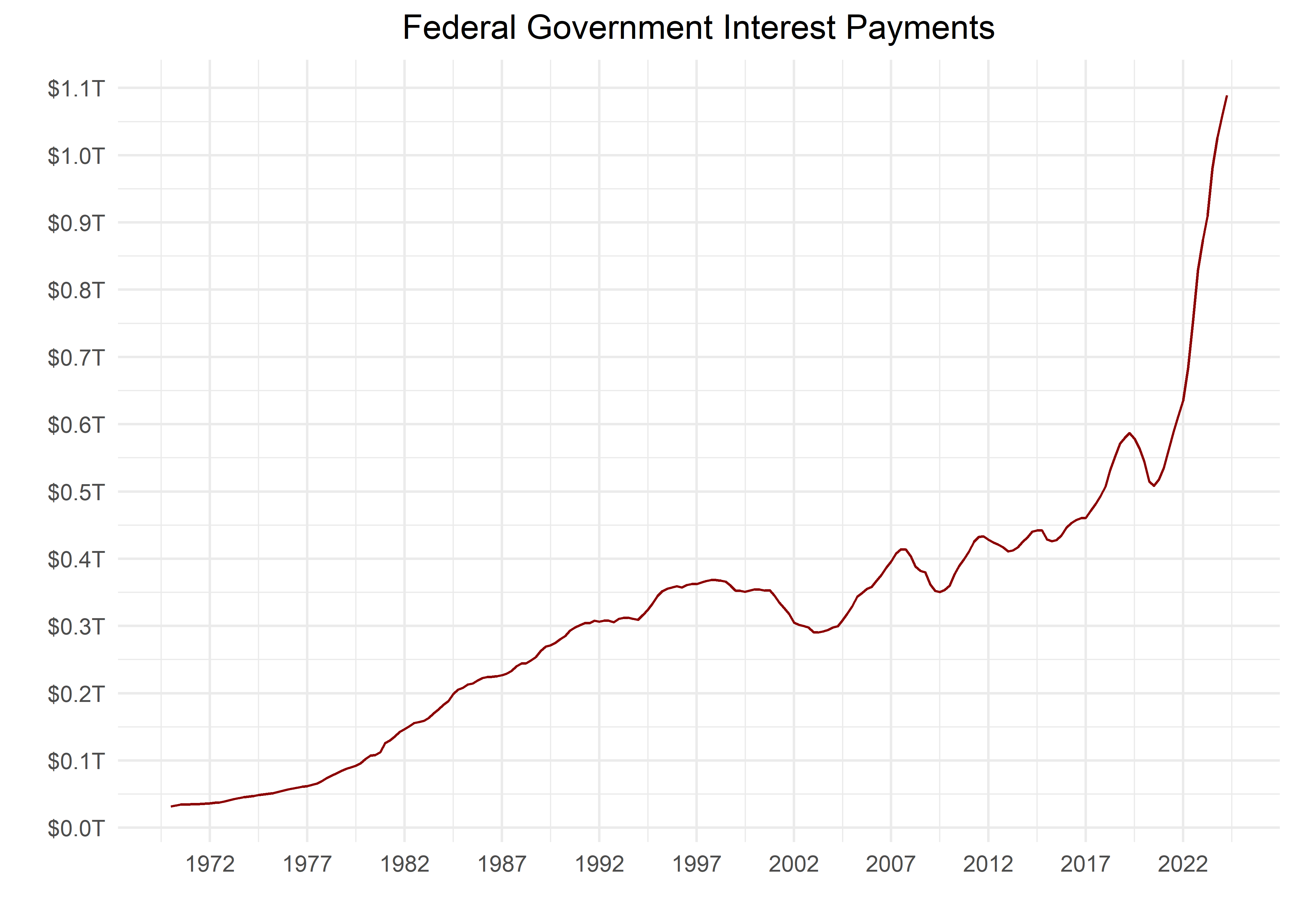
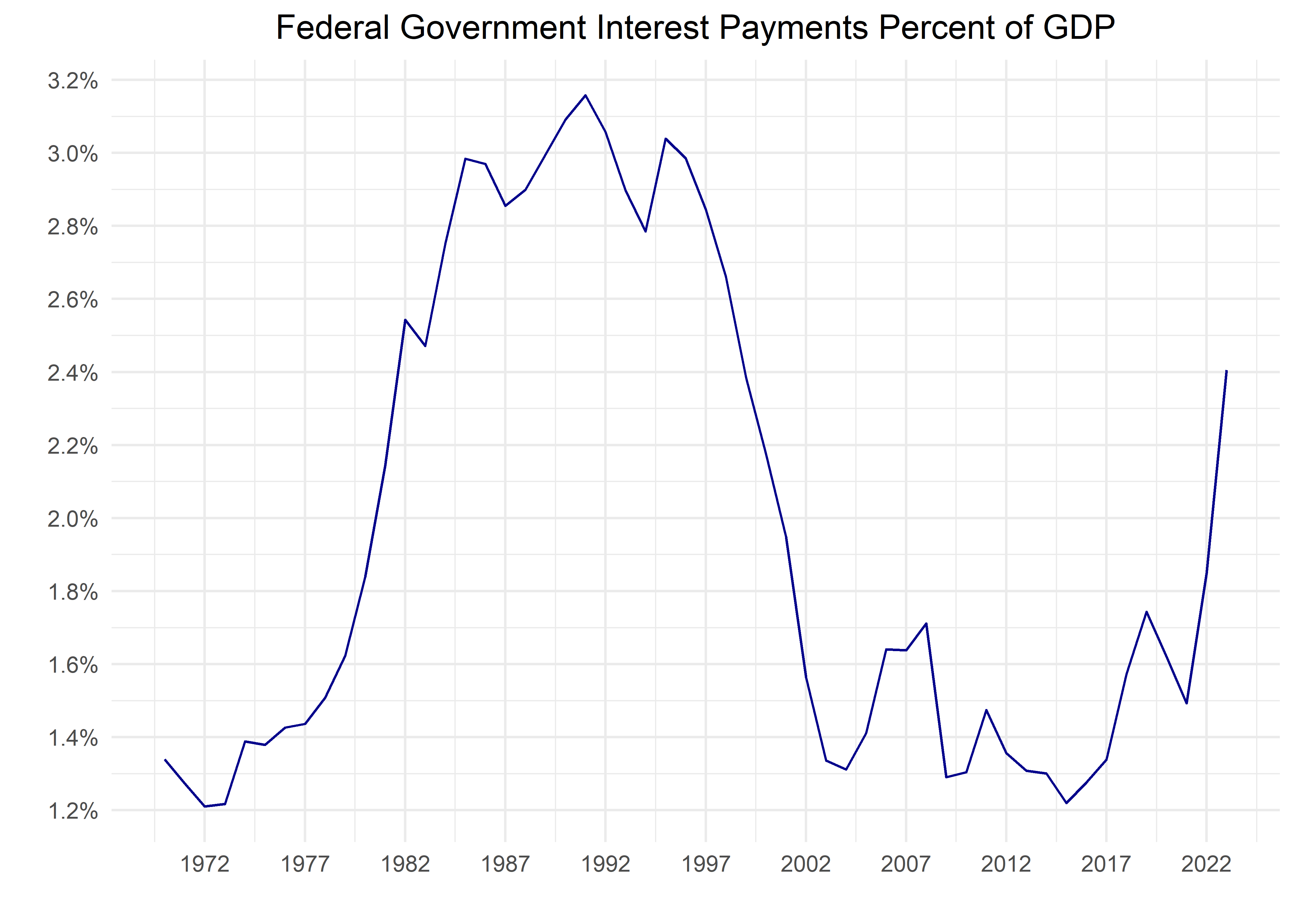
Again, it’s interest rates that set the cost of this debt, and the cost determines how many dollars must be paid to service this debt.

"A091RC1Q027SBEA" %>%
  tq_get(
    get = "economic.data",
    from = "1970-01-01"
  ) %>%
  select(date, fed_int_pymts = price) %>%
  ggplot(aes(
    x = date,
    y = fed_int_pymts
  )) +
  geom_line(color = "darkred") +
  labs(
    x = "",
    y = "",
    title = "Federal Government Interest Payments"
  ) +
  scale_y_continuous(
    labels = dollar_format(
      scale = 1 / 1000,
      accuracy = .1,
      suffix = "T"
    ),
    breaks = pretty_breaks(10)
  ) +
  scale_x_date(
    date_breaks = "5 years",
    date_labels = "%Y"
  ) +
  theme_minimal() +
  theme(plot.title = element_text(hjust = .5))

"FYOIGDA188S" %>%
  tq_get(
    get = "economic.data",
    from = "1970-01-01"
  ) %>%
  select(date, fed_int_pymts = price) %>%
  ggplot(aes(
    x = date,
    y = fed_int_pymts
  )) +
  geom_line(color = "darkblue") +
  labs(
    x = "",
    y = "",
    title = "Federal Government Interest Payments Percent of GDP"
  ) +
  scale_y_continuous(
    labels = percent_format(scale = 1),
    breaks = pretty_breaks(10)
  ) +
  scale_x_date(
    date_breaks = "5 years",
    date_labels = "%Y"
  ) +
  theme_minimal() +
  theme(plot.title = element_text(hjust = .5))

With that, let’s get into interest rates.

Here are the packages we will be using in this chapter:

# workhorse packages
library(tidyverse)
library(tidyquant)
library(timetk)
library(readxl)
library(janitor)

# data sources
library(fredr)
library(riingo)

# vis specific
library(gt)
library(gtExtras)
library(ggrepel)
library(ggtext)
library(plotly)
library(scales)
library(formattable)

How are interest rates set?

Now let’s consider how interest rates come to be at a certain level. A good starting point is the Federal Reserve (the Fed), the central bank of the United States. The Federal Open Market Committee (FOMC) meets eight times a year to determine the federal funds target rate (upper and lower bounds). The Federal Funds or Fed Funds Rate (the FFR) is the interest rate at which depository institutions trade federal funds (balances held at Federal Reserve Banks) with each other overnight. When a depository institution has surplus balances in its reserve account at the Fed, it can lend to other banks that may need larger reserve balances.

The interest rate for borrowing reserve is negotiated by the lender and borrower banks. The weighted average rate for all of these fed funds borrowing is called the effective federal funds rate. The effective federal funds rate is a market determined rate. But it is influenced by the Federal Reserve through open market operations so that it stays in the target federal funds rate range set by FOMC. More specifically, the Federal Reserve decreases liquidity by selling government bonds, reducing the availability of fed funds and thereby raising the federal funds rate. Similarly, the Federal Reserve can increase the availability of fed funds, thereby decreasing the federal funds rate.

The FFR becomes a floor for other interest rates in the econonomy. So even though businesses and homeowners don’t pay the FFR, they in effect pay a spread to the FFR for their commercial bank loans and mortgages.

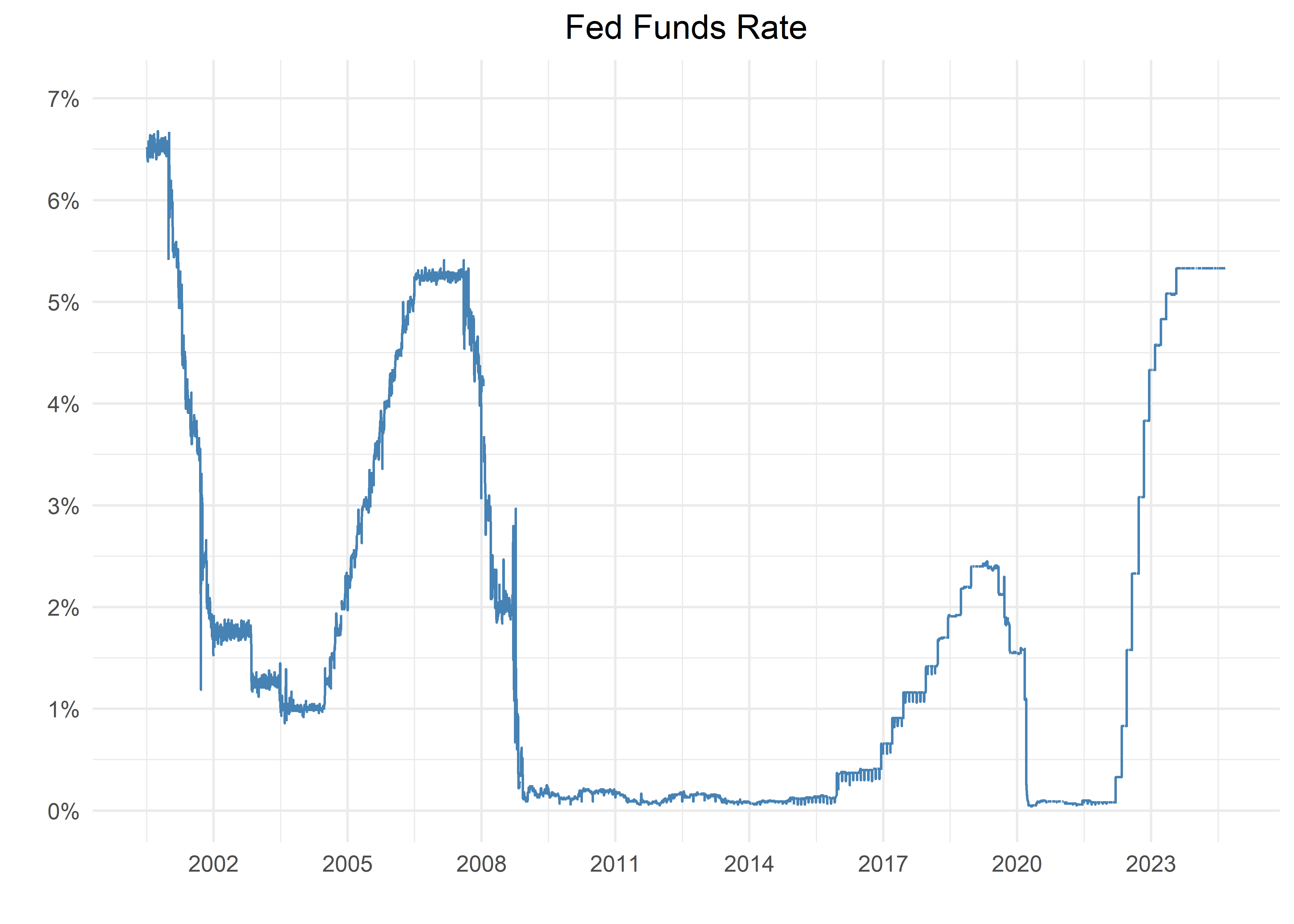
Here is a look at the history of the FFR.

"EFFR" %>%
  tq_get(
    get = "economic.data",
    from = "2000-01-01"
  ) %>%
  ggplot(aes(x = date, y = price)) +
  geom_line(color = "steelblue") +
  labs(
    x = "", y = "",
    title = "Fed Funds Rate"
  ) +
  scale_y_continuous(
    labels = percent_format(
      scale = 1,
      accuracy = 1
    ),
    breaks = pretty_breaks(10)
  ) +
  scale_x_date(
    date_breaks = "3 years",
    date_labels = "%Y"
  ) +
  theme_minimal() +
  theme(plot.title = element_text(hjust = .5))

Treasury Instruments

Data Import and Visualization

Monthly Rates

Interest Rates and Market Returns

Adding Lags

Rolling Features

Putting GDP, Market Data and Treasury Rates together

Exploring relationships

Interest Rate Use Cases

Yield Curve

Dr. Copper and Interest Rates

The CAPE and Interest Rates

Conclusion

Footnotes

See “The Price of Time”, by Edward Chancellor for more background on interest rates in general throughout history.↩︎
See https://media.economist.com/sites/default/files/pdfs/A_Template_for_Understanding\_-\_Ray_Dalio\_\_Bridgewater.pdf.↩︎
See https://www.oaktreecapital.com/insights/memo/sea-change.↩︎
See https://www.oaktreecapital.com/insights/memo/sea-change.↩︎