import yfinance as yf

sp_500_daily = ( yf.download('VFINX',
                      start = '1979-01-01')
                  .reset_index()
)Markets
Introduction
In this chapter, we will import daily stock market price data directly into Python and then wrangle that daily price data into various return series, including future returns. We will also cover some exploratory visualizations that make use of the tools covered in the previous chapter. We also explore a more advanced use case, where we color returns by whether they occurred in a bear market or a bull market. If you are new to coding, the bear market section might be too involved but for the brave it offers a programmatic way to identify market regimes. Let’s get to work on market data.
Obtaining Data: Yahoo! Finance and Polygon
We begin our market data journey with a section on importing and wrangling market data. There are many sources to obtain market data, however when we consider free (or free-ish) accessible sources the number shrinks rapidly. Perhaps the most popular source for free market data is Yahoo! Finance, which can be easily accessed in Python with the yfinance library, and our favorite paid data service is Polygon which offers an application programming interface (API) and has limited free access.
Importing Price Data from Yahoo! Finance
Yahoo! Finance is a great free resource, and yfinance makes it a snap to pull information. However, from time to time the data in Yahoo! Finance suffers changes and revisions which may not be well documented. For this reason, industry professionals use paid services such as Polygon; however, as a free resource, Yahoo! Finance is hard to beat.
For the majority of this book we will source our data from Yahoo! Finance because it is free, quick, and the yfinance library is quite efficient. Pulling data is straightforward: we just use the download method to pass the ticker and date.
For the remainder of this book we will use the S&P 500 as a proxy for the market, and we use the VFINX mutual fund as a price proxy for the S&P 500 because VFINX has a long history, back to the 1970’s, and it is a tradeable instrument. Another traded instrument that tracks the S&P 500 index is the SPY exchange traded fund, however, this asset was created in 1993 and thus has a shorter history. We will use the VFINX as the proxy for the stock market but if you wish to experiment with different assets or funds, it should be smooth to change that ticker. The block of code below pulls the price for the VFINX starting in 1979,
sp_500_daily.head() Date Open High ... Close Adj Close Volume
0 1980-01-02 14.34 14.34 ... 14.34 4.508337 0
1 1980-01-03 14.27 14.27 ... 14.27 4.486334 0
2 1980-01-04 14.45 14.45 ... 14.45 4.542925 0
3 1980-01-07 14.49 14.49 ... 14.49 4.555499 0
4 1980-01-08 14.78 14.78 ... 14.78 4.646671 0
[5 rows x 7 columns]Note that the information provided by Yahoo! Finance is more than just the closing price. We have the date,trading volume, open, high, low, close, and adjusted close prices. Importantly, Yahoo! Finance provides us with adjusted closing prices, these are fictitious prices that include the impact of dividend payments, thus computing percent changes in these adjusted prices would correctly account for the impact of dividends on returns. On the one hand, this adjustment makes our life easier because we can compute accurate returns without worrying about if or when dividends were paid; on the other hand, we do not have true market prices which are needed many times (such as when computing price ratios). The close price does not account for the impact of dividends, thus if we needed to compute price ratios (such as price-to-earnings or price-to-sales) this is the column we use.
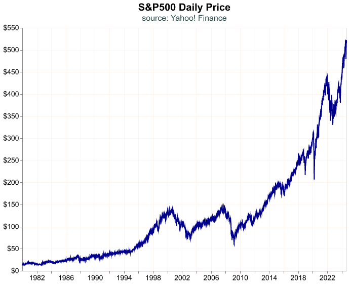
Let’s make a quick chart that shows the closing price over time, note how we format the y-axis so we can make explicit that we are plotting a dollars figure.
(
alt.Chart(sp_500_daily,
    title = alt.Title(
      'S&P500 Daily Price',
      subtitle = 'source: Yahoo! Finance'))
   .mark_line()
   .encode(
      alt.X('Date:T').title(None),
      alt.Y('Close:Q').title(None)
        .axis(format='$.0f')
   )
)
For most of this book and for a lot of macro work, we will not be working with daily prices or even daily returns. Instead we work with weekly, monthly, quarterly or annual returns, so we next turn to transforming daily prices to different periods of returns. Since we need returns, we’ll use the adjusted close column. This is a great example of an idea that is very simple to conceive of in our heads but can get tedious without a smooth code pattern in our toolkit. But before we move on to this task, let’s quickly see how we can obtain price information from Polygon.
